
Why We Stopped Adding Compute and Started Reading the EXPLAIN Plan
When a Redshift cluster starts slowing down, the instinctive reaction is to add more compute. We took a different approach — understanding what was actually happening on the cluster before making any decisions.
"Adding nodes is the loudest fix. Reading the plan is the cheapest one."
Step 1 — Identifying the Heaviest Queries
The starting point was SYS_QUERY_HISTORY, a system view that records all queries executed on the cluster along with metrics such as execution time, queue wait time, and the amount of data returned.
We started by looking at which queries were taking the longest to run on a daily basis:
SELECT
    query_text,
    username,
    datum,
    SUM(minutes) AS query_minutes,
    COUNT(*) AS number_of_exec
FROM (
    SELECT
        u.usename AS username,
        query_type,
        execution_time,
        LEFT(start_time, 10) AS datum,
        elapsed_time / 1000000 / 60 AS minutes,
        query_text
    FROM sys_query_history
    JOIN pg_user u ON user_id = usesysid
    ORDER BY execution_time DESC
)
GROUP BY 1, 2, 3
ORDER BY query_minutes DESC;
This gives a straightforward view of outliers — queries that are individually expensive regardless of how often they run. When we looked at the results, 5 out of the 10 longest-running queries on any given day were materialized view refreshes. That immediately told us where to focus.
To quantify the refresh times, we pulled performance statistics directly from sys_mv_refresh_history:
SELECT
    mv_name,
    MIN(dur_sec) AS min_sec,
    MAX(dur_sec) AS max_sec,
    ROUND(AVG(dur_sec), 1) AS avg_sec
FROM (
    SELECT
        mv_name,
        status,
        start_time,
        end_time,
        duration / 1000000 AS dur_sec
    FROM sys_mv_refresh_history
    WHERE schema_name = 'public'
    ORDER BY start_time
)
GROUP BY mv_name;
This confirmed the problem clearly — refresh times were inconsistent and regularly spiking. We had a measurable baseline to work against.
Step 2 — What the EXPLAIN Plan Reveals
Once we identified materialized view refreshes as a primary source of cluster load, the next step was to look at how those refreshes were actually executing. Running EXPLAIN on the materialized view definition gives the execution plan Redshift uses during refresh — without actually running it.
The plan for our central materialized view looked like this:
XN HashAggregate  (cost=122467142451.64..122496853089.65 rows=276378028 width=152)
  -> XN Hash Join DS_BCAST_INNER  (cost=4249.26..122441153419.28 rows=693040863 width=152)
       Hash Cond: ("outer".account_id = "inner".account_id)
       -> XN Seq Scan on f_transactions a  (cost=0.00..8725658.50 rows=690945069 width=143)
            Filter: (((tx_type)::text <> 'TYPE_G'::text) AND (is_test IS NULL))
       -> XN Hash  (cost=3399.41..3399.41 rows=339941 width=25)
            -> XN Seq Scan on d_accounts dca  (cost=0.00..3399.41 rows=339941 width=25)
Two details immediately stood out.
- DS_BCAST_INNER — Redshift broadcasts the entire
d_accountstable to every compute node because the join column is not a distribution key. This is not a catastrophe on its own, but it becomes expensive in combination with the next problem. - 693 million rows in the join — the join and the entire aggregation with all
CASEexpressions were running directly against the raw transactions table. Every refresh was scanning the full dataset from scratch.
Step 3 — Separating Aggregation from Business Logic
The previous approach was a single materialized view that did everything — join, aggregation, and all business logic (CASE expressions, classifications):
CREATE MATERIALIZED VIEW public.mv_transactions
SORTKEY(tx_date)
DISTKEY(client_id)
AS
SELECT
    a.client_id,
    dca.account_type,
    dca.currency,
    a.location,
    a.tx_date::date,
    CASE
        WHEN a.tx_type = 'TYPE_A' THEN 'Category A'
        WHEN a.tx_type = 'TYPE_B' THEN 'Category B'
        WHEN a.tx_type = 'TYPE_C' THEN 'Category C'
        WHEN a.tx_type IN ('TYPE_E', 'TYPE_F') THEN 'Category D'
        WHEN a.tx_type = 'TYPE_D' THEN 'Category B'
        ELSE 'N/A'
    END AS category,
    a.tx_type AS transaction_type,
    CASE
        WHEN a.tx_sub_type <> '' THEN a.tx_sub_type
        ELSE a.tx_type
    END AS transaction_sub_type,
    CASE
        WHEN a.tx_type IN ('TYPE_E', 'TYPE_F') THEN 'Category D'
        WHEN a.tx_type = 'TYPE_C' THEN 'Category C'
        ELSE a.provider_code
    END AS provider_code,
    CASE
        WHEN a.application = 'TYPE_B' THEN 'Subcategory A'
        WHEN a.tx_type = 'TYPE_E' THEN 'Inflow ' || COALESCE(a.application, '')
        WHEN a.tx_type = 'TYPE_F' THEN 'Outflow ' || COALESCE(a.application, '')
        WHEN a.tx_type = 'TYPE_C' THEN NVL(a.application, 'TYPE_C')
        ELSE COALESCE(a.gid::varchar, a.application)
    END AS application,
    SUM(CASE
        WHEN tx_type = 'TYPE_A' AND tx_canceled = 0 THEN 1
        WHEN tx_type = 'TYPE_A' AND tx_canceled = 1 THEN -1
        WHEN tx_type = 'TYPE_B' AND tx_sub_type = 'TYPE_A' AND tx_canceled = 0 THEN 1
        WHEN tx_type = 'TYPE_B' AND tx_sub_type = 'TYPE_A' AND tx_canceled = 1 THEN -1
        WHEN tx_type = 'TYPE_E' AND tx_canceled = 0 THEN 1
        WHEN tx_type = 'TYPE_E' AND tx_canceled = 1 THEN -1
        ELSE 0
    END) AS tx_count,
    ROUND(SUM(CASE
        WHEN tx_type = 'TYPE_E' THEN amount_in
        WHEN tx_type <> 'TYPE_F' THEN amount_out
        ELSE 0
    END), 2) AS amount,
    ROUND(SUM(CASE
        WHEN tx_type = 'TYPE_F' THEN amount_out
        WHEN tx_type <> 'TYPE_E' THEN amount_in
    END), 2) AS return_amount,
    ROUND(SUM(a.tax_amount), 2) AS tax_amount,
    a.instance
FROM f_transactions a
JOIN d_accounts dca ON a.account_id = dca.account_id
WHERE a.tx_type <> 'TYPE_G'
  AND a.is_test IS NULL
GROUP BY 1,2,3,4,5,6,7,8,9,10,15;
The new approach splits this into two layers.
Layer 1 — Staging Materialized View (Aggregation Only)
CREATE MATERIALIZED VIEW public.stage_mv_transactions
SORTKEY(tx_date)
DISTKEY(client_id)
AS
SELECT
    fat.client_id,
    fat.account_id,
    fat.location,
    fat.terminal,
    fat.deposit_terminal,
    fat.tx_date::date AS tx_date,
    fat.tx_type,
    fat.tx_sub_type,
    fat.tx_canceled,
    fat.provider_code,
    fat.application,
    fat.gid,
    fat.instance,
    fat.deposit_location,
    COUNT(*) AS cnt,
    SUM(fat.amount_out) AS amount_out,
    SUM(fat.amount_in)  AS amount_in,
    SUM(fat.tax_amount) AS tax_amount
FROM f_transactions fat
WHERE fat.tx_type <> 'TYPE_G'
GROUP BY 1,2,3,4,5,6,7,8,9,10,11,12,13,14;
This view knows nothing about business logic. It groups raw transactions and sums amounts — nothing more. The result is a compact dataset of around 12 million rows instead of 693 million.
Layer 2 — Regular View (All Business Logic Applied to Aggregated Data)
CREATE OR REPLACE VIEW public.v_transactions AS
SELECT
    a.client_id,
    dca.account_type,
    dca.currency,
    a.location,
    CASE
        WHEN a.tx_type IN ('TYPE_E', 'TYPE_F') THEN COALESCE(a.deposit_terminal, a.terminal)
        ELSE a.terminal
    END AS terminal,
    a.tx_date AS tx_date,
    CASE
        WHEN a.tx_type = 'TYPE_A' THEN 'Category A'
        WHEN a.tx_type = 'TYPE_B' THEN 'Category B'
        WHEN a.tx_type = 'TYPE_C' THEN 'Category C'
        WHEN a.tx_type IN ('TYPE_E', 'TYPE_F') THEN 'Category D'
        WHEN a.tx_type = 'TYPE_D' THEN 'Category B'
        ELSE 'N/A'
    END AS category,
    a.tx_type AS transaction_type,
    CASE
        WHEN a.tx_sub_type <> '' THEN a.tx_sub_type
        ELSE a.tx_type
    END AS transaction_sub_type,
    CASE
        WHEN a.tx_type IN ('TYPE_E', 'TYPE_F') THEN 'Category D'
        WHEN a.tx_type = 'TYPE_C' THEN 'Category C'
        ELSE a.provider_code
    END AS provider_code,
    CASE
        WHEN a.application = 'TYPE_B' THEN 'Subcategory A'
        WHEN a.tx_type = 'TYPE_E' THEN 'Inflow ' || COALESCE(a.application, '')
        WHEN a.tx_type = 'TYPE_F' THEN 'Outflow ' || COALESCE(a.application, '')
        WHEN a.tx_type = 'TYPE_C' THEN COALESCE(a.application, 'TYPE_C')
        ELSE COALESCE(a.gid::varchar, a.application)
    END AS application,
    SUM(CASE
        WHEN a.tx_type = 'TYPE_A' AND a.tx_canceled = 0 THEN  a.cnt
        WHEN a.tx_type = 'TYPE_A' AND a.tx_canceled = 1 THEN -a.cnt
        WHEN a.tx_type = 'TYPE_B' AND a.tx_sub_type = 'TYPE_A' AND a.tx_canceled = 0 THEN  a.cnt
        WHEN a.tx_type = 'TYPE_B' AND a.tx_sub_type = 'TYPE_A' AND a.tx_canceled = 1 THEN -a.cnt
        WHEN a.tx_type = 'TYPE_E' AND a.tx_canceled = 0 THEN  a.cnt
        WHEN a.tx_type = 'TYPE_E' AND a.tx_canceled = 1 THEN -a.cnt
        ELSE 0
    END) AS tx_count,
    ROUND(SUM(CASE
        WHEN a.tx_type = 'TYPE_E' THEN a.amount_in
        WHEN a.tx_type <> 'TYPE_F' THEN a.amount_out
        ELSE 0
    END), 2) AS amount,
    ROUND(SUM(CASE
        WHEN a.tx_type = 'TYPE_F' THEN a.amount_out
        WHEN a.tx_type <> 'TYPE_E' THEN a.amount_in
        ELSE NULL
    END), 2) AS return_amount,
    ROUND(SUM(a.tax_amount), 2) AS tax_amount,
    a.instance
FROM stage_mv_transactions a
JOIN d_accounts dca ON a.account_id = dca.account_id
GROUP BY
    a.client_id, dca.account_type, dca.currency, a.location, a.tx_date,
    a.tx_type, a.tx_sub_type, a.provider_code, a.application,
    a.gid, a.instance, a.deposit_terminal, a.terminal;
The EXPLAIN plan for the new approach confirms the difference:
XN HashAggregate  (cost=122380381599.54..122380965006.67 rows=4965167 width=163)
  -> XN Hash Join DS_BCAST_INNER  (cost=4249.26..122379883576.78 rows=12450569 width=163)
       Hash Cond: ("outer".account_id = "inner".account_id)
       -> XN Seq Scan on stage_mv_transactions  (cost=0.00..124129.17 rows=12412917 width=154)
       -> XN Hash  (cost=3399.41..3399.41 rows=339941 width=25)
            -> XN Seq Scan on d_accounts dca  (cost=0.00..3399.41 rows=339941 width=25)
DS_BCAST_INNER is still there — the join column is still not a distribution key, and that has not changed. But the outer table in the join now has 12.4 million rows instead of 693 million. Same pattern, drastically different workload.
Step 4 — Incremental Refresh
Both materialized views refresh incrementally — Redshift does not re-read the entire source table from scratch but processes only the rows that are new or changed since the last refresh.
This is not the default behaviour and it matters more than it might seem: without incremental refresh, every run would scan all 700 million rows in the source table, which would largely negate the performance gains from the restructuring in Step 3. A materialized view must satisfy specific conditions documented by AWS, and we structured our queries to meet those requirements.
To verify that a refresh is actually running incrementally, we query sys_mv_refresh_history and check the status:
SELECT
    mv_name,
    status,
    COUNT(*)
FROM sys_mv_refresh_history
WHERE schema_name = 'public'
GROUP BY 1, 2;
A status of Refresh successfully updated MV incrementally confirms that Redshift is performing an incremental refresh rather than a full recompute.
Results
| Scenario | Refresh time |
|---|---|
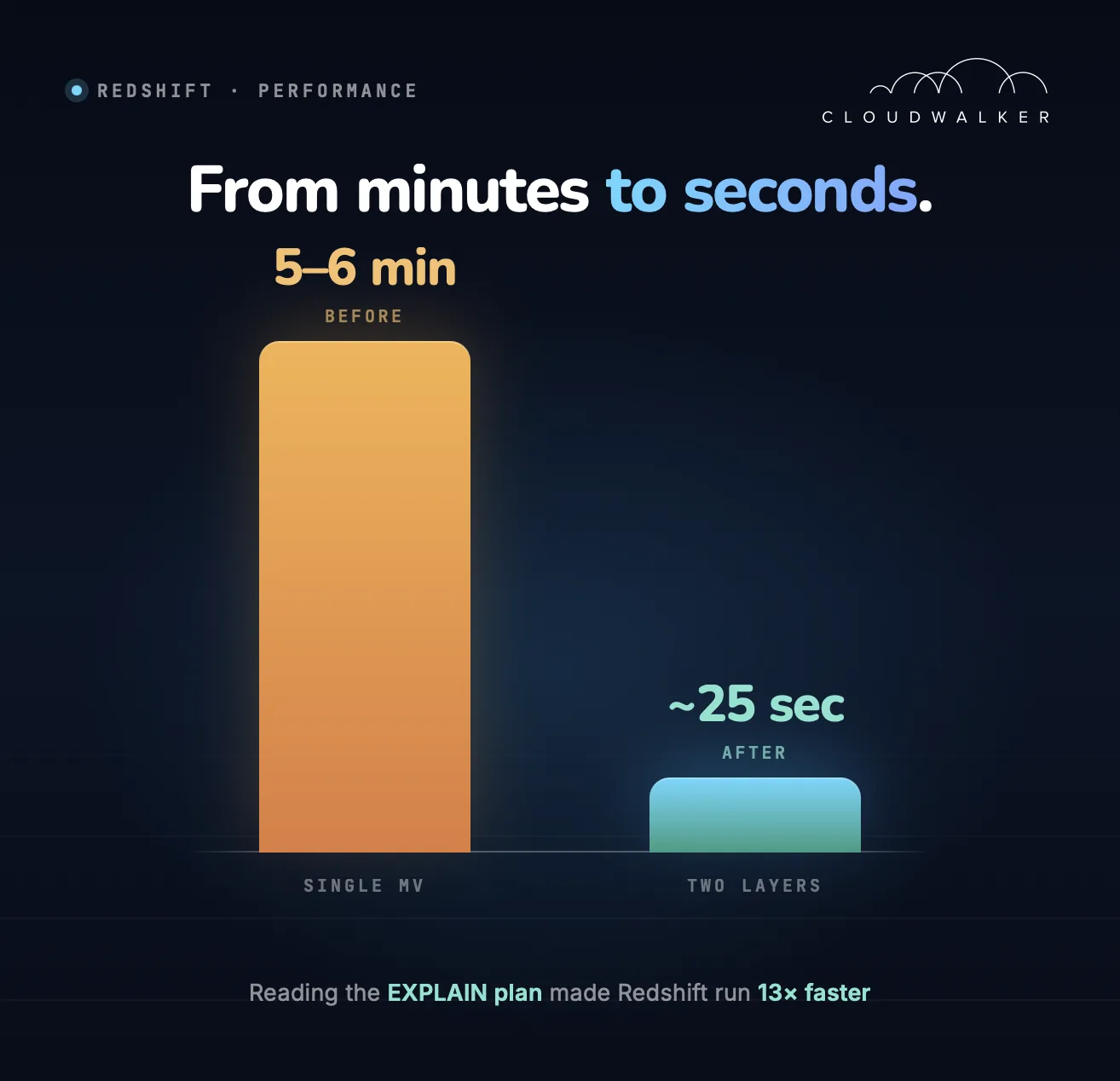
| Before (normal load) | 5–6 minutes |
| Before (cluster under load) | Up to 20 minutes |
| After (staging MV + regular view, incremental) | ~25 seconds |
The cluster load dropped noticeably, refresh became predictable, and analytical services stopped competing with background processes for resources.
Keeping transformation logic out of materialized views and pushing it downstream to regular views means your storage layer stays lean, refreshes stay fast, and business logic remains easy to change without touching the underlying aggregation. When something goes wrong, the separation also makes it much easier to know exactly where to look.
Summary
When Redshift slows down, resist the reflex to scale out. The EXPLAIN plan tells you what's actually expensive — and very often the answer is a query you can restructure, not a cluster you need to grow.
- Measure first. Use
SYS_QUERY_HISTORYandsys_mv_refresh_historyto find what's actually hot. - Read the plan.
DS_BCAST_INNERon a 700M-row table is a flag; the same broadcast on 12M rows is fine. - Separate concerns. Aggregation belongs in materialized views. Business logic belongs in regular views on top of them.
- Verify incremental refresh. The status field in
sys_mv_refresh_historytells you whether Redshift is doing the cheap thing or the expensive thing.